One-Way ANOVA in Python: A Worked Total Bill Example

A real worked analysis using pandas, SciPy, Seaborn, and Statsmodels.

Project type: Python statistics assignment and data visualization

Related help: Data Science Homework Help

Student privacy: The student’s name, university, grade, and deadline are not published.

This project tests whether the mean restaurant bill changes across Thursday, Friday, Saturday, and Sunday in Seaborn’s tips dataset. The submitted Python notebook returns F = 2.7675 and p = 0.04245, so the one-way ANOVA rejects equal means at the 5% level. Tukey’s HSD test then finds no individual day pair significant after adjustment. That difference between the omnibus test and the pairwise follow-up is the central statistical lesson.

Exercise 1: Define the research question before writing the test

The categorical variable is day, with four groups: Thur, Fri, Sat, and Sun. The numeric response is total_bill, which records the bill amount for each observation.

The research question is:

Do average total bills differ across the four days of the week in the Seaborn Tips dataset?

The project notes sometimes refer to comparing tip amounts, but the executed notebook uses df["total_bill"] in the group extraction, ANOVA, Tukey test, and plots. This article follows the code and reports the actual analysis: total bill by day.

The hypotheses are:

• Null hypothesis, H₀: The mean total bill is the same for Thursday, Friday, Saturday, and Sunday.
• Alternative hypothesis, H₁: At least one day has a different population mean total bill.

The significance level is α = 0.05. A one-way ANOVA tests all four means together. It does not identify the specific day that differs, so a significant result requires a follow-up comparison.

Exercise 2: Load and preview the Tips dataset

The notebook loads the example dataset through Seaborn, removes missing rows, and prints the first 10 observations.

import pandas as pd
import seaborn as sns
import matplotlib.pyplot as plt
from scipy.stats import f_oneway, levene, shapiro
from statsmodels.stats.multicomp import pairwise_tukeyhsd

df = sns.load_dataset("tips")
df = df.dropna()

print(df.head(10))

The preview contains these fields:

Column	Meaning	Role in this analysis
total_bill	Total restaurant bill	Numeric response
tip	Tip amount	Available, but not tested here
sex	Reported sex of the customer	Not used in the ANOVA
smoker	Smoker status	Not used in the ANOVA
day	Day of the week	Four-level grouping variable
time	Lunch or dinner	Not used in the ANOVA
size	Party size	Not used in the ANOVA

Seaborn documents load_dataset() as a way to load its example datasets into a pandas DataFrame. The tips dataset is useful for teaching because it combines a numeric bill field with several categorical fields that support different questions. In this project, day supplies the four independent groups and total_bill supplies the response.

Exercise 3: Explore the bill distribution before testing means

The notebook creates a histogram for total_bill and a boxplot for total bill by day.

plt.figure(figsize=(6, 4))
plt.hist(df["total_bill"], bins=20)
plt.title("Histogram of Total Bill")
plt.xlabel("Total Bill")
plt.ylabel("Frequency")
plt.show()

plt.figure(figsize=(6, 4))
sns.boxplot(x="day", y="total_bill", data=df)
plt.title("Total Bill by Day")
plt.show()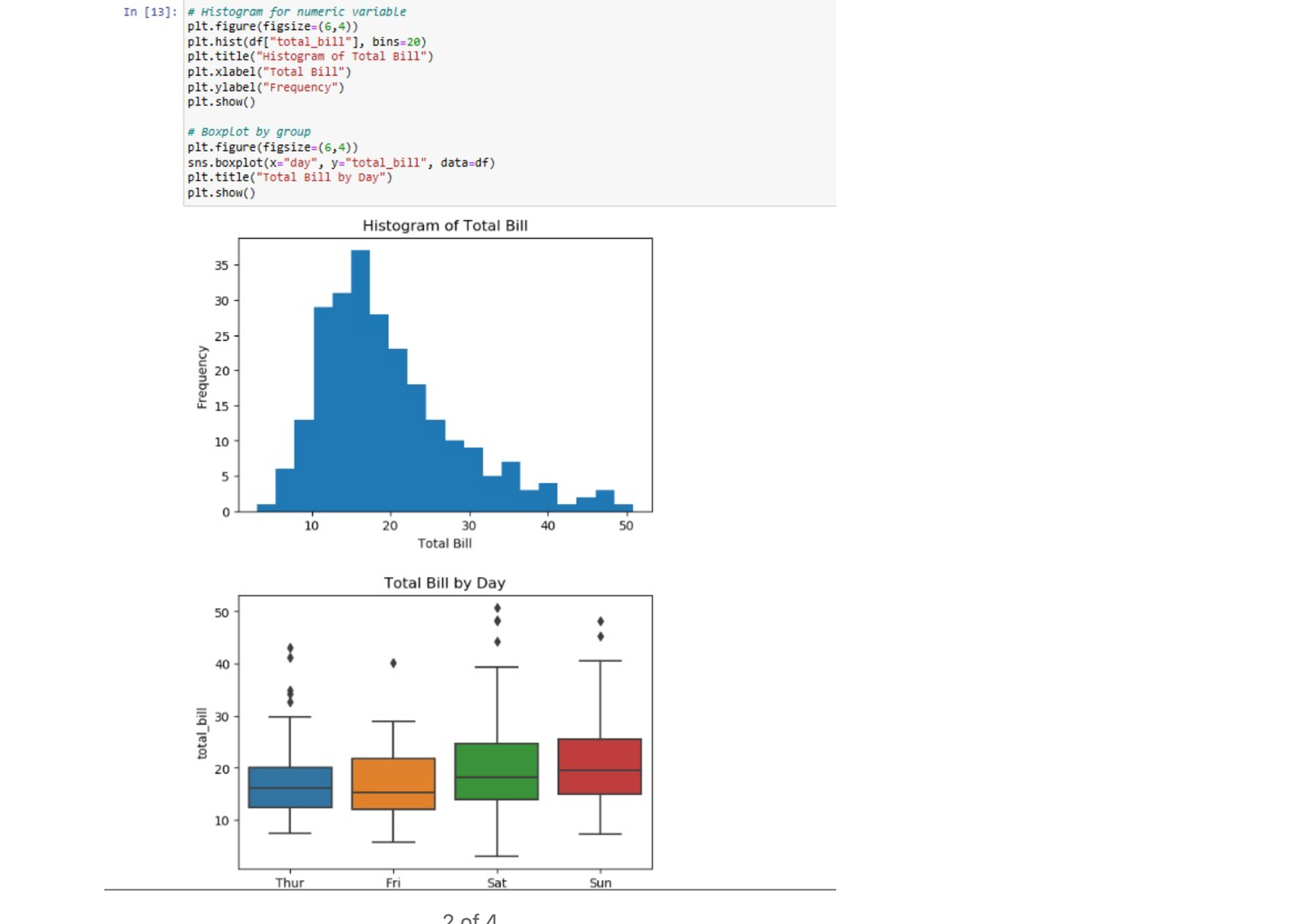

Project screenshot 1. The histogram has a right tail, and the boxplot shows high-value observations in several day groups.

The histogram is concentrated around lower bill values and stretches toward bills above 40. The boxplot shows that the Saturday and Sunday groups have higher central values than Thursday and Friday in the displayed sample, but the boxes overlap. Several points sit beyond the upper whiskers, so the group distributions are not perfectly symmetric.

The visual check does not decide the ANOVA by itself. It tells the analyst which assumptions require numerical checks and which conclusions need cautious wording.

Exercise 4: Check normality and equal variances

The notebook applies a Shapiro-Wilk test within each day group.

groups = [group["total_bill"].values
          for name, group in df.groupby("day")]

for name, group in df.groupby("day"):
    stat, p = shapiro(group["total_bill"])
    print(f"Shapiro-Wilk Normality Test for {name}: p = {p}")

The recorded p-values are:

Day	Shapiro-Wilk p-value	Reading at α = 0.05
Thursday	0.0000286	Evidence against normality
Friday	0.0408565	Evidence against normality
Saturday	0.0000080	Evidence against normality
Sunday	0.0035660	Evidence against normality

All four p-values are below 0.05, so the normality tests reject the within-group normality assumption. The result agrees with the skew and outliers visible in the plots. A Shapiro-Wilk test is not a substitute for checking the plot, and neither test proves that the analysis is unusable. It does establish a limitation: the standard ANOVA result requires a more careful interpretation than it would receive from four roughly normal groups.

The notebook then checks variance homogeneity with Levene’s test.

stat, p = levene(*groups)
print("Levene's Test for Equal Variances: p =", p)

The output is p = 0.574079. Because this value is above 0.05, the analysis does not reject the equal-variance assumption. The variance check supports the standard one-way ANOVA more than the normality check does.

The independence assumption comes from how the observations were collected. The notebook does not test independence, so the final report should avoid claiming that a statistical test proved it. The correct statement is that independence remains a design assumption for this dataset.

Exercise 5: Run the one-way ANOVA in SciPy

The group extraction creates one numeric array for each day. scipy.stats.f_oneway then compares the four group means.

f_stat, p_value = f_oneway(*groups)
print("ANOVA F-statistic:", f_stat)
print("ANOVA p-value:", p_value)

The submitted notebook returns:

ANOVA F-statistic: 2.7674794432863363
ANOVA p-value: 0.04245383328952047

The p-value is below 0.05, so the analysis rejects H₀. The sample contains evidence that the four population means are not all equal. This result does not mean that every day differs, and it does not say which day drives the result. It only says that the four means are unlikely to show this pattern under a model in which all population means are equal.

SciPy describes f_oneway as a test of the null hypothesis that two or more groups have the same population mean. The function returns the F statistic and its associated p-value. In this project, the reported F statistic is the ratio of between-day variation to within-day variation under the standard one-way ANOVA calculation. SciPy’s f_oneway documentation provides the function definition and assumptions.

Exercise 6: Compare the day means visually

The notebook adds a group-mean bar chart:

plt.figure(figsize=(6, 4))
df.groupby("day")["total_bill"].mean().plot(kind="bar")
plt.title("Mean Total Bill by Day")
plt.xlabel("Day")
plt.ylabel("Mean Total Bill")
plt.show()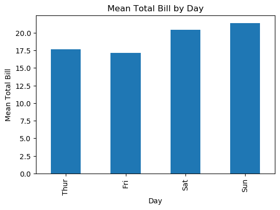

Figure 1. The displayed group means are highest on Sunday and lowest on Friday, with Saturday above both Thursday and Friday.

The bar chart makes the sample pattern easy to read, but it does not replace the inferential test. A taller bar does not automatically mean that the corresponding population mean differs significantly from another bar. The ANOVA evaluates the four means jointly, and Tukey’s HSD controls the error rate when the analysis examines all six day pairs.

Exercise 7: Use Tukey’s HSD to locate pairwise differences

Because the omnibus ANOVA is significant, the notebook runs Tukey’s honestly significant difference test at α = 0.05.

tukey = pairwise_tukeyhsd(
    endog=df["total_bill"],
    groups=df["day"],
    alpha=0.05
)

print(tukey)

The recorded output is:

Group 1	Group 2	Mean difference	Adjusted p-value	Reject H₀?
Fri	Sat	3.2898	0.4554	No
Fri	Sun	4.2584	0.2373	No
Fri	Thur	0.5312	0.9000	No
Sat	Sun	0.9686	0.8921	No
Sat	Thur	-2.7586	0.2375	No
Sun	Thur	-3.7273	0.0669	No

Every reject value is False. The closest comparison is Sunday versus Thursday, with an adjusted p-value of 0.0669. That value is below 0.10 but above the project’s 0.05 threshold, so the Tukey analysis does not declare the pair statistically significant.

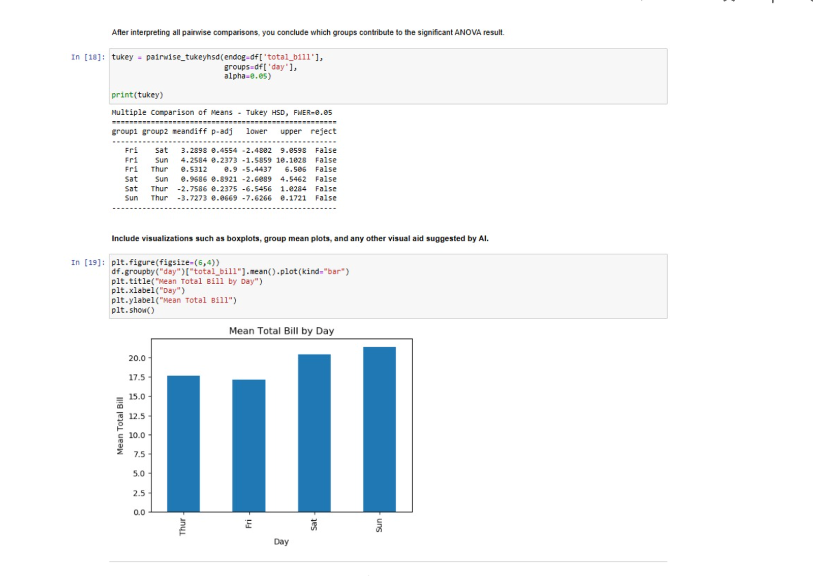
Project screenshot 2. The raw Tukey table reports six adjusted pairwise comparisons, all with reject = False, alongside the mean chart.

Statsmodels documents pairwise_tukeyhsd as a multiple-comparison procedure that returns adjusted p-values. Tukey’s test is stricter than reading six unadjusted comparisons because it controls the family-wise error rate across the set of pairwise tests. Statsmodels’ Tukey HSD documentation describes the endog, groups, and alpha arguments used here.

Why the ANOVA is significant while Tukey finds no pair

The two results answer related but different questions.

The ANOVA asks whether the four means can be treated as equal as a group. Its p-value is 0.04245, which crosses the 0.05 threshold. Tukey’s HSD asks six separate pairwise questions while controlling the chance of at least one false positive across the full set. Its adjusted p-values are larger, and none falls below 0.05.

This pattern is possible when the means show a broad day-level signal, the groups overlap, and the correction reduces the evidence for any single pair. It is not a coding error and it does not justify choosing Sunday versus Thursday as a significant result. The defensible conclusion is narrower:

The one-way ANOVA detects an overall difference among day means at the 5% level, but the Tukey HSD follow-up does not identify a statistically significant pair at the same level.

The project also reports non-normal group distributions. A stronger extension would compare the standard ANOVA with a Welch ANOVA or a rank-based alternative, explain the independence design, and report an effect size with a confidence interval. Those additions would extend the analysis; they do not change the reported results from the submitted code.

What this Python analysis teaches

The valuable part of the project is the order of the work:

1. Define the grouping variable and response variable.
2. State H₀ and H₁ before reading the p-value.
3. Inspect the distributions with a histogram and boxplot.
4. Check normality and equal variances.
5. Run the omnibus ANOVA.
6. Use Tukey’s HSD only after a significant omnibus result.
7. Interpret the full set of outputs together.

That sequence prevents three common errors. It stops the analyst from calling a bar-chart gap proof of significance. It stops the analyst from claiming that ANOVA identifies a specific pair. It also stops the report from hiding assumption checks after the conclusion.

AI supported the project by suggesting a dataset, helping shape the research question, explaining the tests, and providing coding guidance. The submitted notebook still contains the actual variable choices, test calls, outputs, and plots. Mrinal S.’s expert-led explanation keeps the interpretation tied to those outputs rather than presenting AI text as statistical evidence.

Common questions about this ANOVA solution

Is this an ANOVA of tips or total bills?

It is an ANOVA of total_bill by day. The dataset contains a tip column, but the executed notebook passes total_bill to f_oneway, pairwise_tukeyhsd, and the charts.

What does p = 0.04245 mean?

It means the observed four-group pattern has a probability of about 4.25% under the null model that all population means are equal, assuming the model’s conditions and the sampling design are appropriate. It is not the probability that the null hypothesis is true.

Which day has the highest average bill?

Sunday has the tallest bar in the submitted mean chart, while Friday has the shortest. The descriptive ordering does not create a statistically significant Tukey pair at α = 0.05.

Does a significant ANOVA prove that every day differs?

No. It shows that at least one population mean differs somewhere among the groups. The Tukey output is required to examine the individual pairs.

Did the normality assumption pass?

No. All four Shapiro-Wilk p-values are below 0.05, and the plots show skew and outliers. Levene’s test for equal variances passed with p = 0.574079. The final write-up should report both facts.

Is the code correct even though Tukey finds no significant pair?

Yes. The code answers two different statistical questions correctly: f_oneway tests the four means jointly, and pairwise_tukeyhsd performs adjusted pairwise comparisons. Different conclusions at those two levels are statistically possible.

Expert and source note

This worked solution was written by Mrinal S., Python Expert from the supplied ANOVA requirement, Code.ipynb, report, and project screenshots. The data source is the Seaborn tips example dataset, and the statistical functions are documented by SciPy and Statsmodels. Students working on similar Python analysis assignments can explore Python Learning Resources or visit the DoMyPythonHomework homepage.