Python NumPy and Logistic Regression: A CS549 Assignment

A worked explanation of the supplied Python notebook, including NumPy exercises, SAT-to-GPA regression, sign-language image classification, and the checks that make the results reproducible.

Project type: Python and NumPy machine learning assignment

Related help: NumPy Homework Help

Student privacy: The student’s name, university, grade, and deadline are not published.

This CS549 assignment combines Python and NumPy practice with two machine-learning implementations. The first model predicts university GPA from Math SAT and Verbal SAT scores. The second model classifies two encoded sign-language image groups with logistic regression. In the supplied notebook, the image classifier reports 94.06% training accuracy and 88.00% test accuracy, with an F1 score of 0.8872 on the held-out test set.

The most useful part of the project is the path from a blank code cell to a tested result. The notebook implements the mathematics directly with NumPy instead of hiding the work inside a high-level machine-learning library. If you are working through a similar brief, our python programming assignment help page is a relevant place to discuss the exact part of the code that is blocking you.

Quick facts from the supplied assignment

Project component	What the supplied files contain
Course and assignment	CS549 Machine Learning assignment
Python and NumPy section	4 exercises worth 20 points
Linear regression section	Normal equation, gradient descent, and learning-rate comparison
Logistic regression section	7 implementation tasks worth 40 points
GPA dataset	105 rows with Math SAT, Verbal SAT, and GPA values
Image data	2,062 images, each 64 x 64 pixels, with 10 encoded label positions
Binary image subset	Encoded label positions 0 and 6 in the runnable code
Image feature matrix	4,096 features per image after flattening
Held-out image test set	125 examples
Reported test accuracy	88.00%

The last two rows describe the notebook’s saved run, not a universal performance claim. The result belongs to this dataset, this class-selection rule, this 70/30 split, this learning rate, and this implementation.

What the assignment asks students to build

The assignment asks students to complete code cells marked with None or TODO, run evaluation cells, and make the output match the expected values. It has three connected sections:

1. Python and NumPy exercises: strings, loops, vectorized comparisons, reshaping, slicing, transposing, and matrix multiplication.
2. Linear regression: a normal-equation solution and a gradient-descent solution for predicting GPA from two SAT features.
3. Logistic regression: a binary image classifier built from the sigmoid function through gradient descent, prediction, accuracy, precision, recall, and F1 score.

The assignment also expects written understanding. A good explanation names the array shapes, describes the loss function, explains why normalization matters, and interprets the test metrics instead of listing numbers without context.

For students planning the work from the beginning, our Python setup guide pairs well with this project because the notebook needs Python, Jupyter, NumPy, Matplotlib, and scikit-image in the same working environment.

The NumPy skills behind the notebook

NumPy stores numerical data in ndarray objects. An array has a shape, and that shape controls which operations are valid. A one-dimensional vector with 16 values can become a 4 x 4 matrix without changing the values:

import numpy as np

arr = np.arange(1, 17)
arr_reshaped = arr.reshape(4, 4)
middle_columns = arr_reshaped[:, 1:3]

print(arr_reshaped.sum())
print(arr_reshaped.mean())

The supplied output is a total sum of 136 and a mean of 8.5. The slice [:, 1:3] selects every row and columns 1 and 2. Python starts indexing at zero, so these are the second and third visible columns.

The notebook also uses the matrix multiplication operator. For the matrix below, the transpose and matrix product produce the expected 2 x 2 result:

A = np.array([[1, 2], [3, 4], [5, 6]])
result = A.T @ A

[[35 44]
 [44 56]]

This operation appears again in the normal-equation solution. Understanding the dimensions before writing the formula prevents many NumPy errors.

Four short exercises and their evidence

The first task reverses the string I love Python with a loop and counts vowels and consonants. The supplied evaluation output is:

Reversed string: nohtyP evol I
Vowel count: 4
Consonant count: 7

The second task creates a 3 x 3 matrix with numpy.random.randn, counts entries greater than or equal to 0.5, and locates them with numpy.argwhere. With numpy.random.seed(0), the count is 5 and the five positions are:

[[0 0]
 [0 2]
 [1 0]
 [1 1]
 [2 0]]

The fixed seed matters. Without it, the matrix and the expected positions change each time the cell runs.

The final NumPy exercise calculates A.T @ A. It demonstrates three ideas that carry into the regression sections: an array has a declared shape, transpose changes the orientation, and matrix multiplication differs from element-by-element multiplication.

Linear regression: predicting GPA from SAT scores

The linear-regression dataset contains 105 rows with three unnamed columns: Math SAT, Verbal SAT, and university GPA. The supplied values range from 516 to 718 for Math SAT, 480 to 732 for Verbal SAT, and 2.08 to 3.81 for GPA.

The notebook normalizes each column by its maximum value:

data = np.loadtxt(open("sat_gpa.csv"), delimiter=",")
data_norm = data / data.max(axis=0)

This is a simple scale adjustment. It places the features and target on comparable numerical ranges before gradient descent. The notebook uses all 105 rows as training data, so the exercise demonstrates implementation and optimization rather than out-of-sample GPA forecasting.

Building the design matrix

The regression design matrix contains an intercept column followed by the two normalized SAT features:

X = np.ones_like(data_norm)
X[:, 1:3] = data_norm[:, 0:2]
y = data_norm[:, 2]

The first column of ones allows the model to learn an intercept. Each row of X contains one student’s two SAT values, and y contains the normalized GPA for that row.

Normal equation and residual error

The normal equation computes the parameter vector directly:

theta = np.linalg.inv(X.T @ X) @ X.T @ y
y_hat = X @ theta
RSS = np.sum((y - y_hat) ** 2)

The supplied notebook reports:

Result	Value
Intercept	-0.06234478
Math SAT coefficient	0.62017319
Verbal SAT coefficient	0.43647674
Residual sum of squares	0.7590471383

The coefficient signs describe the fitted relationship on the normalized data. They do not mean that GPA changes by the same raw number of points for every one-point SAT increase because the features were scaled first.

For a production implementation, numpy.linalg.solve is usually preferable to explicitly forming an inverse. The assignment asks students to use the inverse, so the notebook follows that instruction.

Gradient descent and vectorized updates

The second solution starts with theta equal to [0, 0, 0] and updates all three parameters repeatedly. The update is vectorized through the design matrix:

def gradient_descent(X, y, theta, alpha, num_iters):
    m = len(y)
    costs = []

    for _ in range(num_iters):
        y_hat = X @ theta
        diff = y_hat - y
        costs.append(np.sum(diff ** 2) / (2 * m))
        gradients = (X.T @ diff) / m
        theta = theta - alpha * gradients

    y_hat = X @ theta
    rss = np.sum((y - y_hat) ** 2)
    return theta, rss, costs

With alpha equal to 0.05 and 500 iterations, the supplied output is:

Result	Value
Intercept	0.29911574
Math SAT coefficient	0.32224209
Verbal SAT coefficient	0.31267172
Residual sum of squares	0.8641600584

The gradient-descent RSS is higher than the normal-equation RSS in this run. That difference is an important discussion point. The normal equation solves the least-squares system directly, while gradient descent stops after a fixed number of steps. A different learning rate, more iterations, or a stopping rule based on the change in cost can move the iterative solution closer to the direct solution.

What the learning-rate plots show

The notebook tests alpha values 0.01, 0.005, and 0.002. Each cost curve decreases, but the larger learning rate reaches a low cost sooner. The smallest rate decreases more gradually across the 500 iterations.

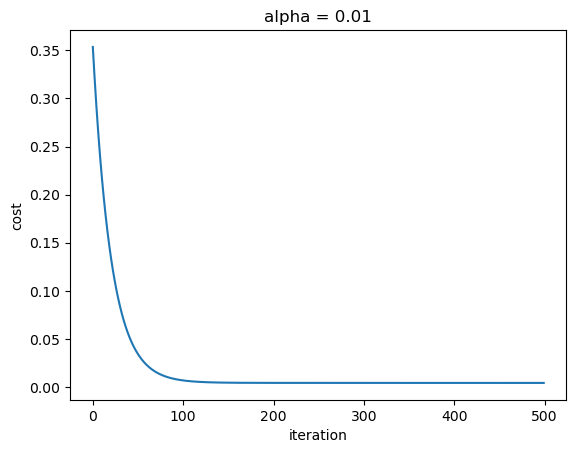
Figure 1. With alpha = 0.01, the cost falls quickly and levels off near the end of the run.

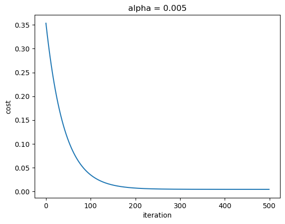
Figure 2. With alpha = 0.005, the descent remains stable but takes longer to approach the low-cost region.

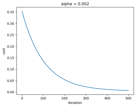
Figure 3. With alpha = 0.002, the curve is still descending at iteration 500.

These plots answer the assignment’s learning-rate question without pretending that one value is universally best. The useful choice depends on scale, iteration budget, and whether the curve decreases smoothly instead of oscillating or diverging.

Logistic regression: classifying two image groups

The second machine-learning section implements logistic regression from the ground up. The archive contains X.npy, Y.npy, and an lc.png learning-curve image. The notebook loads the image tensor and one-hot labels, flattens each 64 x 64 image into 4,096 features, selects two encoded label groups, and converts the task into binary labels 0 and 1.

The saved run reports these shapes:

X_raw shape: (2062, 64, 64)
Y_raw shape: (2062, 10)
X_data shape: (4096, 2062)
Y_data shape: (1, 2062)
X_train shape (4096, 286)
Y_train shape (1, 286)
X_test shape (4096, 125)
Y_test shape (1, 125)

The code selects encoded label positions 0 and 6. The notebook’s explanatory text calls the classes signs “three” and “four,” but the executable selection is Y_data == 0 and Y_data == 6. The dataset documentation or label mapping must confirm those names before the assignment is described as a specific three-versus-four classifier. This article keeps the code-level description visible so the result remains traceable.

The split takes the first 70 percent of each selected group for training and the remaining 30 percent for testing. That produces 286 training examples and 125 test examples. Because the code does not shuffle before slicing, the ordering of the source data affects the split. A stronger experiment uses a stratified, seeded split after checking that the source ordering is not correlated with collection conditions.

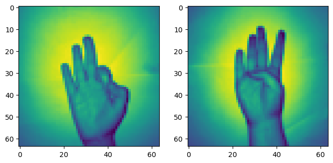
Figure 4. The notebook displays one example from each selected encoded class before training the classifier.

The sigmoid function

Logistic regression converts a linear score into a value between zero and one with the sigmoid function:

def sigmoid(z):
    return 1 / (1 + np.exp(-z))

The evaluation cell checks sigmoid(-10) and sigmoid(10). The outputs are approximately 0.0000454 and 0.9999546. These values behave like probabilities for the positive class, although a probability becomes a class prediction only after a threshold is applied.

Forward pass, loss, and gradients

The notebook initializes w as a (4096, 1) zero vector and b as 0.0. For one training pass, it computes:

Z = np.dot(w.T, X) + b
A = sigmoid(Z)
cost = (-1 / m) * np.sum(
    Y * np.log(A) + (1 - Y) * np.log(1 - A)
)

dZ = A - Y
dw = (1 / m) * np.dot(X, dZ.T)
db = (1 / m) * np.sum(dZ)

The forward pass produces the predicted probabilities and binary cross-entropy cost. The backward pass calculates the gradient for each of the 4,096 weights and for the bias. The supplied evaluation cell reports dw, db, and a cost of 6.9550195708 for its small test matrix.

For a safer implementation, clip A before calling numpy.log:

eps = 1e-12
A_safe = np.clip(A, eps, 1 - eps)
cost = (-1 / m) * np.sum(
    Y * np.log(A_safe) + (1 - Y) * np.log(1 - A_safe)
)

Clipping prevents log(0) when a large score pushes a sigmoid value to the edge of floating-point precision.

Gradient descent, prediction, and metrics

The GD function calls the forward-backward calculation, updates w and b, and stores one cost value every 100 iterations. The final model uses 1,500 iterations and alpha = 0.002. Its cost decreases from 0.6931471806 at iteration 0 to 0.2634118207 at iteration 1,400.

The prediction step applies a threshold of approximately 0.5:

def predict(X, w, b):
    probabilities = sigmoid(w.T @ X + b)
    return (probabilities >= 0.5).astype(float)

This vectorized version produces the same type of output as the supplied notebook while removing an unnecessary loop that repeatedly reassigns the entire prediction array.

The model then compares predictions with Y_test and calculates the confusion-matrix counts:

Metric	Supplied test result
True positives	59
False positives	11
True negatives	51
False negatives	4
Accuracy	0.8800
Precision	0.842857
Recall	0.936508
F1 score	0.887219

The positive-class recall is higher than precision. In this test set, the classifier finds most of the positive examples, but it also produces 11 false positives. The F1 score balances those two class-specific measures. A student should report the confusion counts with the metrics because accuracy alone hides which error type the model makes.

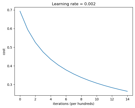
Figure 5. The binary cross-entropy cost decreases across the stored checkpoints in the supplied run.

Reproducibility checks before submission

The notebook reaches the expected outputs, but four details deserve a check before anyone treats it as a reusable classifier.

1. Match the filename case

The notebook calls numpy.load(open(‘y.npy’, ‘rb’)), while the supplied ZIP contains Y.npy with an uppercase Y. Windows often treats those names as equivalent, but case-sensitive systems do not. Rename the file or update the notebook so the code and archive use the same spelling.

2. Confirm the class-label dictionary

The prose and executable code use different descriptions for the selected sign classes. Check the original dataset mapping, then write that mapping in the notebook before presenting the confusion matrix as a named digit comparison.

3. Preserve the training and test protocol

The supplied notebook selects the first 70 percent of each class for training. A reordered source file changes which examples enter the test set. A seeded stratified split makes the experiment easier to reproduce, but it also changes the reported numbers, so the method and result must be reported together.

4. Separate teaching code from production code

The assignment intentionally implements sigmoid, gradients, prediction, and metrics manually. That is the right approach for learning the mathematics. A production classifier adds data validation, stable loss calculations, an explicit random split, saved preprocessing rules, and a repeatable evaluation script.

Students who are stuck on array shapes, file loading, or unexpected NumPy errors can also use our Python common errors resource before changing the model logic.

What this assignment teaches clearly

This project connects small NumPy operations to a complete machine-learning workflow:

• array shape controls matrix multiplication;
• normalization affects the scale seen by gradient descent;
• the normal equation and gradient descent solve the same linear-regression objective in different ways;
• a sigmoid converts a linear score into a probability-like output;
• vectorized gradients remove unnecessary Python loops;
• a 4,096-feature image matrix can be handled as a regular NumPy array;
• accuracy, precision, recall, F1, and confusion counts describe different parts of classifier behavior.

The notebook also teaches a less obvious lesson: an output can match the expected value and still require a reproducibility note. File-name case, class mappings, split order, and numerical stability all affect whether another student can run the same code on another computer.

Questions students often ask

What topics does the CS549 assignment cover?

The CS549 assignment covers Python basics, NumPy array operations, linear regression with the normal equation, linear regression with gradient descent, logistic regression, image flattening, sigmoid activation, binary cross-entropy, parameter updates, prediction thresholds, and classification metrics.

Why does the gradient-descent RSS exceed the normal-equation RSS?

The normal equation solves the least-squares system directly, while the supplied gradient-descent run stops after 500 updates. The iterative result can improve with a different learning rate, more iterations, or a convergence check based on the change in cost.

How many features does each image have after preprocessing?

Each 64 x 64 image becomes a column with 4,096 pixel features after flattening. The training matrix therefore has shape (4096, 286) and the test matrix has shape (4096, 125).

What does the reported 88% test accuracy mean?

It means 110 of the 125 held-out examples receive the correct binary label in the supplied run. The remaining five metrics add detail: 59 true positives, 11 false positives, 51 true negatives, and 4 false negatives.

Is the classifier definitely recognizing signs three and four?

The notebook text says three and four, but the runnable code selects encoded label positions 0 and 6. The original label dictionary must confirm the human-readable class names before that claim is used in a final report.

Why does the assignment avoid a machine-learning library for the core model?

The assignment is testing the mechanics of linear and logistic regression. Implementing the sigmoid, gradient calculations, parameter updates, and metrics with NumPy makes each mathematical step visible. A library implementation is useful later, but it would hide the skills being assessed here.

Final takeaway

The supplied notebook is a solid teaching example because it moves from a 4 x 4 NumPy matrix to two end-to-end learning algorithms. Its strongest evidence is concrete: the normal-equation coefficients, the three learning-rate curves, the 4,096-feature image matrix, the falling logistic cost, and the 88% held-out accuracy.

Its limitations are equally useful. The class-label wording needs verification, the Y.npy filename needs to match the load statement, and the image split depends on source ordering. Documenting those points makes the project more credible and gives students a practical model for writing the discussion section of a Python machine-learning assignment.

If you are working on a similar NumPy or classifier project, our NumPy homework help page and machine learning homework help page cover the two main skill areas in this notebook. You can also start from our python programming assignment help page when the brief combines several Python topics.

Sources and further reading

• Python 3 documentation
• NumPy documentation
• Matplotlib documentation
• scikit-image installation documentation
• Sign Language Digits Dataset repository